

pairs trading using data-driven techniques simple trading strategies part 1
Pairs Trading using Data-Driven Techniques: Simple Trading Strategies Part 3
![]()
Pairs trading is a overnice exercise of a scheme based happening mathematical analysis. We'll demonstrate how to leveraging data to create and automate a pairs trading strategy.
Download Ipython Notebook here.
Underlying Principle
Army of the Righteou's say you have a dyad of securities X and Y that have roughly underlying economic link, for example two companies that manufacture the same product alike Pepsi and Coca Cola. You gestate the ratio or difference in prices (also called the distribute) of these two to remain steadfast with time. Notwithstandin, now and again, on that point might be a divergence in the spread 'tween these two pairs caused past temporary supply/demand changes, large buy/sell orders for one security, chemical reaction for important news about one of the companies etc. In this scenario, one stock moves rising while the former moves down congener to each other. If you expect this divergence to revert gage to normal with time, you toilet make a pairs trade.
When there is a temporary divergence, the pairs trade would be to sell the outperforming stock (the stock that stirred up )and to buy the underperforming blood line (the stock that moved down ). You are making a bet that the spread between the two stocks would eventually converge by either the outperforming standard moving pull out or the underperforming stock moving back up or both — your trade will score money in all of these scenarios. If both the stocks rise or move down together without changing the spread between them, you don't make or fall back whatsoever money.
Therefore, pairs trading is a commercialise neutral trading strategy facultative traders to profit from virtually any market conditions: uptrend, downtrend, Oregon sideways campaign.
Explaining the Concept: We start by generating two fake securities.
                          significance              numpy              as              np
              import              pandas              as              pd                              import                statsmodels
                from                statsmodels.tsa.stattools                significance                coint
                # merely set the seed for the random total source
np.random.seed(107)                              import                matplotlib.pyplot                as                plt
Let's generate a fake security X and model it's daily returns past drawing from a normal distribution. Then we perform a cumulative sum to get the value of X on apiece twenty-four hours.

            # Generate day-after-day returns            Xreturns = np.random.average(0, 1, 100)                        # sum them and shift altogether the prices up            X = pd.Series(np.cumsum(
              Xreturns), name='X')
              + 50
X.plot(figsize=(15,7))
plt.indicate()
At present we generate Y which has a deep worldly data link to X, so price of Y should vary pretty likewise equally X. We model this by winning X, shifting it up and adding some random noise drawn from a normal distribution.
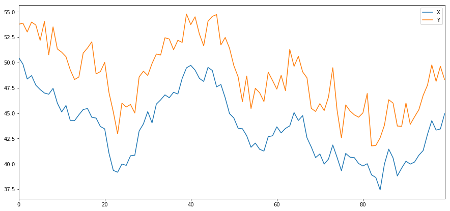
            haphazardness = np.random.normal(0, 1, 100)
Y = X + 5 + noise
Y.name = 'Y'            pd.concat([X, Y], axis=1).plot(figsize=(15,7))            plt.show()
Cointegration
Cointegration, very similar to correlation, means that the ratio between two series bequeath vary approximately a mean. The two series, Y and X follow the follwing:
Y = ⍺ X + e
where ⍺ is the constant ratio and e is white racket. Read more present
For pairs trading to work between two timeseries, the expected value of the ratio over time must converge to the mean, i.e. they should be cointegrated.
The prison term serial publication we constructed above are cointegrated. We'll plot the ratio between the deuce like a sho thus we can regard how this looks.
![]()
            (Y/X).plot(figsize=(15,7))                        plt.axhline((Y/X).mean(), color='violent', linestyle='--')                        plt.xlabel('Fourth dimension')
plt.legend(['Mary Leontyne Pric Ratio', 'Mean'])
plt.show()
Testing for Cointegration
There is a commodious test that lives in statsmodels.tsa.stattools. We should see a identical low p-prise, as we've artificially created two serial publication that are as cointegrated as physically possible.
                          # compute the p-time value of the cointegration examination
              # will inform us as to whether the ratio between the 2 timeseries is stationary
              # some its mean
score, pvalue, _ = coint(X,Y)
              print              pvalue
1.81864477307e-17
Remark: Correlation vs. Cointegration
Correlation and cointegration, while theoretically similar, are not the same. Let's look after at examples of series that are correlated, but not cointegrated, and the other way around. First let's check the correlation of the series we merely generated.
X.corr(Y) 0.951
That's selfsame high, as we would expect. But how would deuce series that are correlated but not cointegrated look? A swordlike example is two series that just vary.
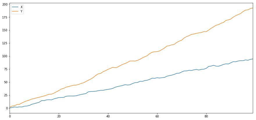
ret1 = np.random.mean(1, 1, 100)
ret2 = Np.random.normal(2, 1, 100)s1 = pd.Serial( nurse clinician.cumsum(ret1), name='X')
s2 = pd.Series( np.cumsum(ret2), name='Y')atomic number 46.concat([s1, s2], axis=1 ).plot(figsize=(15,7))
publish 'Correlation: ' + str(X_diverging.corr(Y_diverging))
plt.present()
score, pvalue, _ = coint(X_diverging,Y_diverging)
print 'Cointegration test p-value: ' + str(pvalue)
Correlational statistics: 0.998
Cointegration try p-value: 0.258
A simple example of cointegration without correlation is a normally distributed serial publication and a square wave.
              Y2 = pd.Serial publication(np.random.formula(0, 1, 800), name='Y2') + 20
Y3 = Y2.transcript() 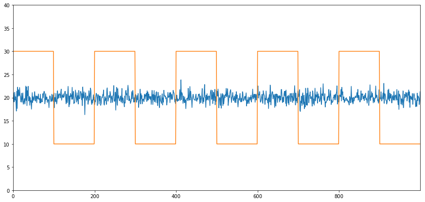
              Y3[0:100] = 30
Y3[100:200] = 10
Y3[200:300] = 30
Y3[300:400] = 10
Y3[400:500] = 30
Y3[500:600] = 10
Y3[600:700] = 30
Y3[700:800] = 10
                            Y2.secret plan(figsize=(15,7))
Y3.plot()
plt.ylim([0, 40])
plt.demonstrate()                              # correlation is well-nigh zero
                black and white                'Correlation coefficient: ' + str(Y2.corr(Y3))
account, pvalue, _ = coint(Y2,Y3)
                print                'Cointegration test p-value: ' + str(pvalue)
Correlational statistics: 0.007546
Cointegration trial p-value: 0.0
The correlation is implausibly low, merely the p-value shows unflawed cointegration!
How to draw a pairs trade?
Because two cointegrated time series (such as X and Y above) swan towards and apart from each other, there will be times when the spread is higher and times when the spread is low. We make a pairs swop away buying one security and selling another. This way, if both securities go down together operating theater go up together, we neither make nor lose money — we are market neutral.
Going back to X and Y higher up that follow Y = ⍺ X + e, such that ratio (Y/X) moves around it's mean ⍺, we make money on the ratio of the two reverting to the mean. In order to do this we'll watch for when X and Y are far apart, i.e ⍺ is as well high or too low:
- Exit Long the Ratio This is when the ratio ⍺ is small than usual and we expect it to increase. In the above deterrent example, we place a bet on this by purchasing Y and selling X.
- Going Snub the Ratio This is when the ratio ⍺ is large and we expect it to get on smaller. In the above example, we direct a wager on this away merchandising Y and purchasing X.
Note that we always possess a "hedged position": a short position makes money if the security sold loses value, and a extended position will make money if a security system gains value, so we're immune to overall market movement. We single make or lose money if securities X and Y move relative to each another.
Using Data to find securities that behave like this
The good way to do this is to start with securities you suspect may be cointegrated and do a statistical essa. If you just run statistical tests over all pairs, you'll fall target to multiple comparison oblique.
Five-fold comparisons bias is simply the fact that on that point is an inflated run a risk to incorrectly generate a significant p-value when many tests are run, because we are running a lot of tests. If 100 tests are run on random data, we should expect to see 5 p-values below 0.05. If you are comparing n securities for co-integration, you will execute n(n-1)/2 comparisons, and you should wait to see umteen incorrectly significant p-values, which bequeath increase Eastern Samoa you increase. To stave off this, pick a microscopic number of pairs you have rationality to suspect might be cointegrated and screen to each one singly. This will solvent in less exposure to multiple comparisons bias.
So Army of the Pure's try to find some securities that display cointegration. Let's crop with a basket of US gigantic cap tech stocks — in Sdanamp;P 500. These stocks operate in a similar segment and could have cointegrated prices. We scan through a list of securities and test for cointegration between all pairs. Information technology returns a cointegration test nock matrix, a p-value intercellular substance, and whatsoever pairs for which the p-value was less than 0.05. This method is inclined to multiple comparison bias and in practice the securities should be subject to a 2d verification step. Let's ignore this for the sake of this object lesson.
              def find_cointegrated_pairs(data):
                n = data.shape[1]
                score_matrix = np.zeros((n, n))
                pvalue_matrix = neptunium.ones((n, n))
                keys = data.keys()
                pairs = []
                for i in range(n):
                for j in scope(i+1, n):
                S1 = data[keys[i]]
                S2 = data[keys[j]]
                result = coint(S1, S2)
                score = result[0]
                pvalue = final result[1]
                score_matrix[i, j] = tally
                pvalue_matrix[i, j] = pvalue
                if pvalue danlt; 0.02:
                pairs.append((keys[i], keys[j]))
                return score_matrix, pvalue_matrix, pairs
Note: We include the market bench mark (SPX) in our data — the market drives the movement of then many securities that often you might find oneself 2 seemingly cointegrated securities; but in reality they are not cointegrated with each strange simply both conintegrated with the market. This is titled a confounding variable and it is important to check for market involvement in whatever relationship you find.
from backtester.dataSource.yahoo_data_source import YahooStockDataSource
from datetime import datetime startDateStr = '2007/12/01'
endDateStr = '2017/12/01'
cachedFolderName = 'yahooData/'
dataSetId = 'testPairsTrading'
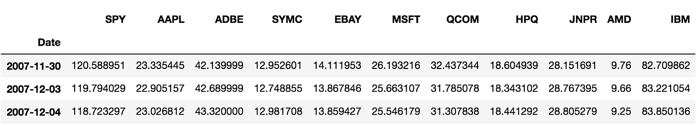
instrumentIds = ['SPY','AAPL','ADBE','SYMC','EBAY','MSFT','QCOM',
'HpQ','JNPR','AMD','IBM']
ds = YahooStockDataSource(cachedFolderName=cachedFolderName,
dataSetId=dataSetId,
instrumentIds=instrumentIds,
startDateStr=startDateStr,
endDateStr=endDateStr,
event='account') information = ds.getBookDataByFeature()['Adj Scalelike'] data.head(3)
Now let's effort to breakthrough cointegrated pairs using our method.
              # Heatmap to show the p-values of the cointegration test
# 'tween each pair of stocks              scores, pvalues, pairs = find_cointegrated_pairs(data)
implication seaborn
m = [0,0.2,0.4,0.6,0.8,1]
seaborn.heatmap(pvalues, xticklabels=instrumentIds,
                yticklabels=instrumentIds, cmap='RdYlGn_r',
                mask = (pvalues dangt;= 0.98))
plt.show up()
print pairs

[('ADBE', 'MSFT')] Looks like 'ADBE' and 'MSFT' are cointegrated. Allow's get a load at the prices to make sure this in reality makes sense.
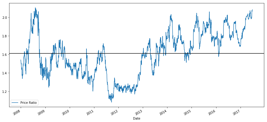
              S1 = data['ADBE']
S2 = data['MSFT']
score, pvalue, _ = coint(S1, S2)
mark(pvalue)
ratios = S1 / S2
ratios.plot()
plt.axhline(ratios.normal())
plt.legend([' Ratio'])
plt.show()
The ratio does look like it moved around a stable mean.The right-down ratio isn't very useful in statistical footing. It is many helpful to normalize our signal aside treating it as a z-score. Z score is defined as:
Z Grade (Value) = (Value — Entail) / Standard Digression
WARNING
In practice this is usually done to try to give some scale to the data, just this assumes an underlying distribution. Usually normal. Notwithstandin, much financial data is non normally distributed, and we must be very careful not to simply assume normality, surgery any specific distribution when generating statistics. The veracious statistical distribution of ratios could be very fat-caudated and prostrate to extreme values messing up our theoretical account and sequent in galactic losses.
                              def                zscore(series):
return (series - series.mean()) / np.std(series) 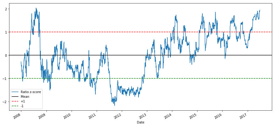
              zscore(ratios).plot()
plt.axhline(zscore(ratios).mean())
plt.axhline(1.0, color='red')
plt.axhline(-1.0, color='leafy vegetable')
plt.show()
It's easier to now observe the ratio now moves around the mean, but sometimes is prone to large divergences from the mean, which we john take advantages of.
Now that we've talked about the basics of pair trading strategy, and identified co-integrated securities based on historical Leontyne Price, let's try to develop a trading signal. First, let's recap the steps in developing a trading signal using data techniques:
- Collect authentic Data and clean Information
- Create features from data to key out a trading signal/logic
- Features lav be moving averages or ratios of price data, correlations or more compound signals — combine these to create new features
- Generate a trading signal victimization these features, i.e which instruments are a buy, a sell or neutral
Step 1: Setup your job
Hera we are trying to make a signal that tells us if the ratio is a bribe or a trade at the next instant in fourth dimension, i.e our prediction adaptable Y:
Y = Ratio is buy (1) or sell (-1)
Y(t)= Sign( Ratio(t+1) — Ratio(t) )
Government note we don't need to augur actual neckcloth prices, or even up actual value of ratio (though we could), just the focusing of next move in ratio
Step 2: Pull in Reliable and Accurate Information
Auquan Toolbox is your friend here! You entirely have to specify the broth you want to swap and the datasource to use, and IT pulls the required data and cleans it for dividends and stock splits. So our data here is already clean.
We are using the following data from Yahoo at every day intervals for trading years over close 10 years (~2500 data points): Open, Close, High, Low and Trading Volume
Stone's throw 3: Split Data
Don't forget this super important step to test accuracy of your models. We're exploitation the favorable Training/Proof/Test Snag
- Training 7 years ~ 70%
- Test ~ 3 years 30%
              ratios = data['ADBE'] / data['MSFT']
print(len(ratios))
train = ratios[:1762]
test = ratios[1762:]
Ideally we should also make a validation set but we volition skip this for at present.
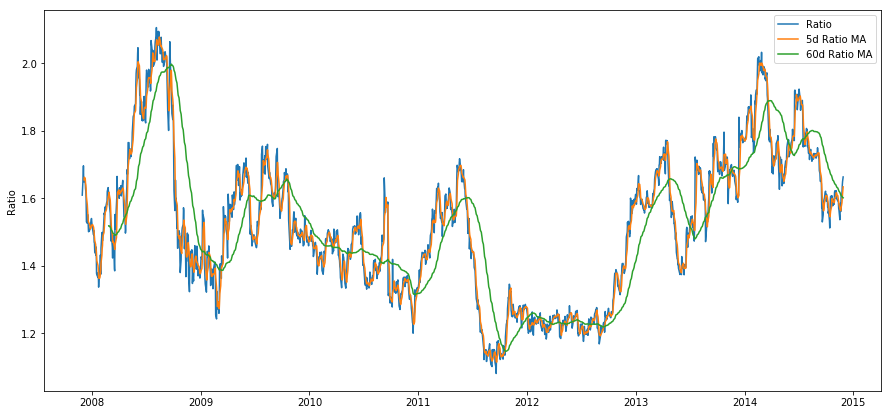
dance step 4: Boast Engineering
What could relevant features be? We want to predict the direction of ratio move. We've seen that our two securities are cointegrated so the ratio tends to turn and revert back to the mean. IT seems our features should be foreordained measures for the mean of the ratio, the divergence of the live value from the mean to be able to generate our trading signal.
Allow's use the following features:
- 60 day Moving Average of Ratio: Measure of rolling mean
- 5 day Moving Average of Ratio: Measure of live esteem of mean
- 60 Clarence Shepard Day Jr. Standard Deviation
- z score: (5d Mommy — 60d MA) /60d SD
              ratios_mavg5 = take.rolling(window=5,
                center=False).mean()              ratios_mavg60 = train.rolling(windowpane=60,
                sum=False).mean()              std_60 = train.resonating(window=60,
                center=False).std()              zscore_60_5 = (ratios_mavg5 - ratios_mavg60)/std_60
plt.figure(figsize=(15,7))
plt.plot(train.index finger, aim.values)
plt.plot(ratios_mavg5.index, ratios_mavg5.values)
plt.plat(ratios_mavg60.index, ratios_mavg60.values)              plt.legend(['Ratio','5d Ratio MA', '60d Ratio MA'])              plt.ylabel('Ratio')
plt.bear witness()
              plt.figure out(figsize=(15,7))
zscore_60_5.plat()
plt.axhline(0, discolour='black')
plt.axhline(1.0, color='red', linestyle='--')
plt.axhline(-1.0, color='green', linestyle='--')
plt.legend(['Rolling Ratio z-Score', 'Mean', '+1', '-1'])
plt.evidenc() 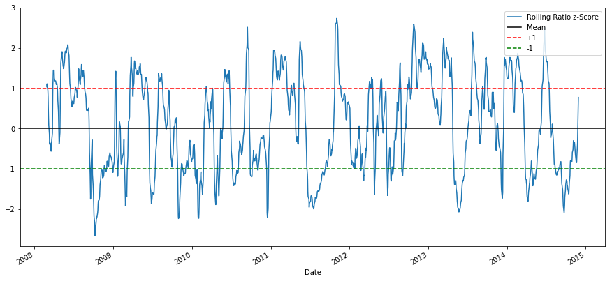
The Z Score of the rolling means really brings unconscious the mean reverting nature of the ratio!
Step 5: Model Selection
Let's start with a really simple posture. Looking at the z-make graph, we tush see that whenever the z-score feature gets too high, or too low, it tends to revert back. Let's use +1/-1 as our thresholds for likewise high and too low, then we can use the following simulation to generate a trading signal:
- Ratio is buy (1) whenever the z-grade is below -1.0 because we bear z nock to go back up to 0, hence ratio to gain
- Ratio is betray(-1) when the z-score is above 1.0 because we gestate z score to recuperate down to 0, hence ratio to decrease
Stair 6: Train, Validate and Optimize
Finally, LET's see how our model actually does connected real information? Let's see what this signal looks like connected actual ratios
              # Plot the ratios and bribe and sell signals from z grudge
plt.figure(figsize=(15,7))              train[60:].plot()
buy = train.copy()
trade = train.re-create()
buy[zscore_60_5dangt;-1] = 0
sell[zscore_60_5danlt;1] = 0
buy[60:].plot(color='g', linestyle='None', marker='^')
sell[60:].plot(color='r', linestyle='None', marking='^')
x1,x2,y1,y2 = plt.axis()
plt.axis((x1,x2,ratios.min(),ratios.max()))
plt.legend(['Ratio', 'Buy Signal', 'Sell Impressive'])
plt.show off()
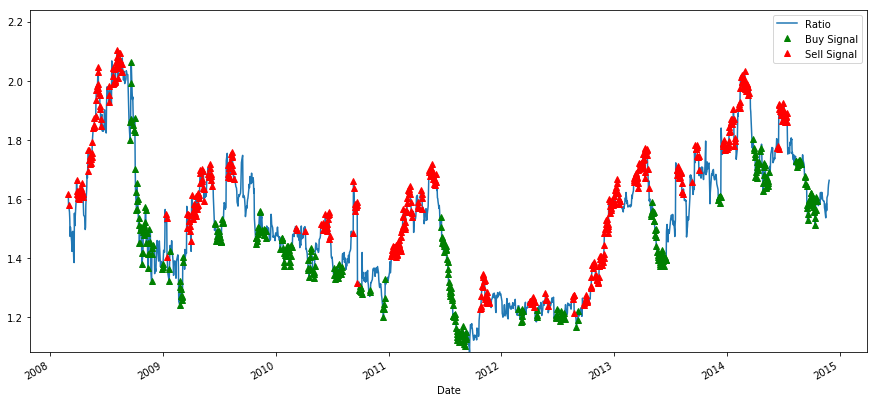
The signalize seems reasonable, we seem to sell the ratio (ruddy dots) when it is high or increasing and grease one's palms it support when it's low (green dots) and decreasing. What does that mean for actual stocks that we are trading? Let's get a load
              # Plot the prices and buy and sell signals from z grudge
plt.figure(figsize=(18,9))
S1 = data['ADBE'].iloc[:1762]
S2 = data['MSFT'].iloc[:1762]              S1[60:].plot(color='b')
S2[60:].plot(color='c')
buyR = 0*S1.copy()
sellR = 0*S1.copy()              # When buying the ratio, buy S1 and deal out S2
buyR[buy!=0] = S1[buy!=0]
sellR[bargain!=0] = S2[buy!=0]
# When selling the ratio, sell S1 and buy S2
buyR[sell!=0] = S2[betray!=0]
sellR[deal out!=0] = S1[deal!=0]              buyR[60:].plat(color='g', linestyle='None', mark='^')
sellR[60:].plot(colour='r', linestyle='No', mark='^')
x1,x2,y1,y2 = plt.axis()
plt.axis((x1,x2,min(S1.min(),S2.min()),max(S1.max(),S2.max())))              plt.legend(['ADBE','MSFT', 'Bribe Signal', 'Deal out Signal'])
plt.show()
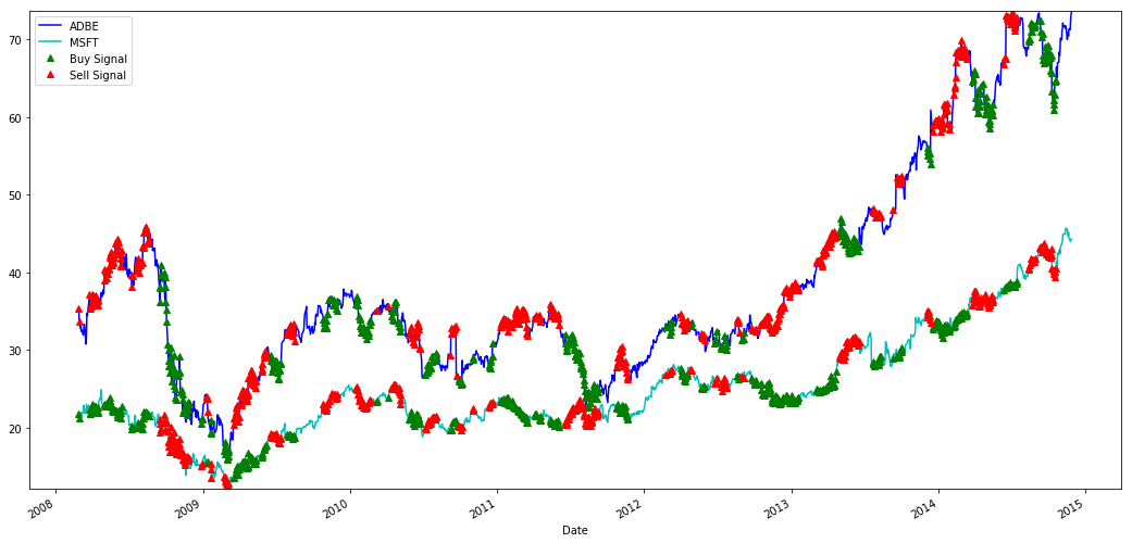
Discover how we sometimes make money connected the short leg and sometimes on the long-acting leg, and sometimes both.
We'atomic number 75 happy with our signal on the training data. Let's see what kind-hearted of profits this signal can generate. We can make a ensiform backtester which buys 1 ratio (buy 1 ADBE stock and sell ratio x MSFT strain) when ratio is dejected, sell 1 ratio (sell 1 ADBE stock and buy ratio x MSFT stock) when information technology's high and calculate PnL of these trades.
# Trade using a simple strategy
def deal out(S1, S2, window1, window2):# If window length is 0, algorithmic rule doesn't make common sense, so pass
if (window1 == 0) or (window2 == 0):
return 0# Reckon rolling ungenerous and rolling received deviation
ratios = S1/S2
ma1 = ratios.rolling(window=window1,
center=False).mean()
ma2 = ratios.roll(window=window2,
nitty-gritty=False).mean()
std = ratios.reverberating(windowpane=window2,
substance=False).std()
zscore = (ma1 - ma2)/std# Sham trading
# Start with no money and nobelium positions
money = 0
countS1 = 0
countS2 = 0
for i in kitchen stove(len(ratios)):
# Betray short if the z-score is dangt; 1
if zscore[i] dangt; 1:
money += S1[i] - S2[i] * ratios[i]
countS1 -= 1
countS2 += ratios[i]
print('Selling Ratio %s %s %s %s'%(money, ratios[i], countS1,countS2))
# Buy long-range if the z-score is danlt; 1
elif zscore[i] danlt; -1:
money -= S1[i] - S2[i] * ratios[i]
countS1 += 1
countS2 -= ratios[i]
print('Buying Ratio %s %s %s %s'%(money,ratios[i], countS1,countS2))
# Clear positions if the z-score between -.5 and .5
elif abs(zscore[i]) danlt; 0.75:
money += S1[i] * countS1 + S2[i] * countS2
countS1 = 0
countS2 = 0
print('Exit pos %s %s %s %s'%(money,ratios[i], countS1,countS2))return money
trade(data['ADBE'].iloc[:1763], information['MSFT'].iloc[:1763], 5, 60)
629.71
So that strategy seems profitable! Now we can optimize further by changing our moving average windows, by changing the thresholds for buy/sell and exit positions etc and stop for performance improvements on validation data.
We could also try more sophisticated models like Logisitic Fixation, SVM etc to make our 1/-1 predictions.
For like a sho, permit's say we decide to go forward with this model, this brings us to
Step 7: Backtest on Psychometric test Information
Backtesting is simple, we can just use our function from above to see PnL on test data
deal(data['ADBE'].iloc[1762:], data['MSFT'].iloc[1762:], 5, 60) 1017.61
The model does quite well! This makes our first elongate pairs trading exemplary.
Avoid Overfitting
Before closing the treatment, we'd look-alike to establish special note to overfitting. Overfitting is the most dangerous booby trap of a trading strategy. An overfit algorithm may perform wonderfully connected a backtest simply fails miserably on new-sprung unseen information — this mean it has not really uncovered any trend in data and nobelium real predictive power. Let's take a simple example.
In our model, we used rolling parameter estimates and may wish to optimize windowpane distance. We may decide to simply retel over all possible, reasonable window length and pick the length supported which our model performs the prizewinning . Below we write a simple loop to to score windowpane lengths founded on pnl of training data and find the best one.
            # Find the windowpane length 0-254
# that gives the highest returns using this scheme
length_scores = [trade(data['ADBE'].iloc[:1762],
              information['MSFT'].iloc[:1762], l, 5)
              for l in range(255)]
best_length = np.argmax(length_scores)
photographic print ('Scoop windowpane duration:', best_length)
('Best window length:', 246) Now we check the performance of our model on essa data and we uncovering that this window length is far from optimal! This is because our original choice was clearly overfitted to the sample information.
            # Find the returns for test information
# using what we think out is the best window distance
length_scores2 = [deal(information['ADBE'].iloc[1762:],
              data['MSFT'].iloc[1762:],l,5)
              for l in range(255)]
print (best_length, 'sidereal day windowpane:', length_scores2[best_length])            # Breakthrough the best window distance supported connected this dataset,
# and the returns using this windowpane length
best_length2 = np.argmax(length_scores2)
print (best_length2, 'day window:', length_scores2[best_length2])
            (1, 'day window:', 10.06)
(218, 'daytime window:', 527.92)
Clearly fitting to our sample information doesn't always give good results in the succeeding. Just for fun, let's plot the length scores computed from the ii datasets
            plt.figure(figsize=(15,7))
plt.diagram(length_scores)
plt.plot(length_scores2)
plt.xlabel('Windowpane length')
plt.ylabel('Score')
plt.caption(['Grooming', 'Quiz'])
plt.express() 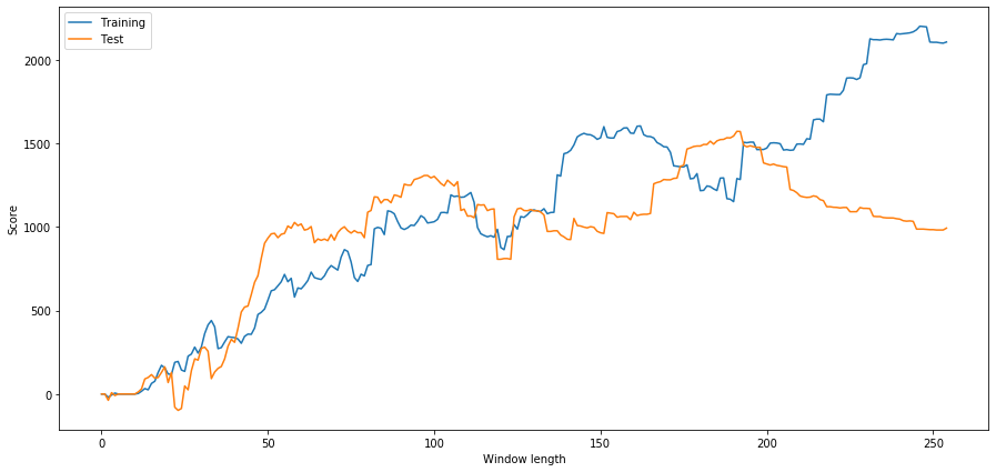
We can see that anything above about 90 would be a effective choice for our window.
To avoid overfitting, we can use economic reasoning or the nature of our algorithm to pick our window duration. We behind too use Kalman filters, which do not require us to specify a length; this method will be covered in another notebook afterward.
Next Steps
In this stake, we bestowed many simple introductory approaches to demonstrate the action of nonindustrial a pairs trading scheme. In practice one should use more sophisticated statistics, some of which are listed here
- Hurst exponent
- Half-life of mean reversion inferred from an Ornstein–Uhlenbeck process
- Kalman filters
pairs trading using data-driven techniques simple trading strategies part 1
Source: https://medium.com/auquan/pairs-trading-data-science-7dbedafcfe5a
Posted by: foxpenated.blogspot.com
0 Response to "pairs trading using data-driven techniques simple trading strategies part 1"
Post a Comment